How to Read 1000 Watt Scale on Dozy Tr1000

Time series is a sequence of observations recorded at regular time intervals. This guide walks you through the process of analyzing the characteristics of a given fourth dimension series in python.

Time Series Analysis in Python – A Comprehensive Guide. Photo by Daniel Ferrandiz.

What is a Fourth dimension Serial?
How to import Time Series in Python?
What is panel data?
Visualizing a Time Series
Patterns in a Fourth dimension Series
Additive and multiplicative Fourth dimension Series
How to decompose a Time Serial into its components?
Stationary and non-stationary Time Series
How to brand a Time Series stationary?
How to test for stationarity?
What is the deviation between white noise and a stationary series?
How to detrend a Fourth dimension Series?
How to deseasonalize a Fourth dimension Series?
How to test for seasonality of a Time Series?
How to treat missing values in a Time Series?
What is autocorrelation and partial autocorrelation functions?
How to compute fractional autocorrelation part?
Lag Plots
How to estimate the forecastability of a Time Series?
Why and How to smoothen a Time Serial?
How to apply Granger Causality test to know if one Time Series is helpful in forecasting another?
What Adjacent

one. What is a Time Series?

Time series is a sequence of observations recorded at regular fourth dimension intervals. Depending on the frequency of observations, a time series may typically be hourly, daily, weekly, monthly, quarterly and annual. Sometimes, you might take seconds and minute-wise time serial every bit well, like, number of clicks and user visits every minute etc. Why fifty-fifty analyze a time series? Because it is the preparatory footstep before you develop a forecast of the series. Besides, time series forecasting has enormous commercial significance because stuff that is of import to a business similar need and sales, number of visitors to a website, stock toll etc are essentially fourth dimension series data. Then what does analyzing a time series involve? Time serial analysis involves understanding diverse aspects about the inherent nature of the serial and then that you are better informed to create meaningful and accurate forecasts.

two. How to import fourth dimension series in python?

And then how to import time series data? The data for a fourth dimension series typically stores in .csv files or other spreadsheet formats and contains two columns: the engagement and the measured value. Let'due south employ the read_csv() in pandas package to read the fourth dimension serial dataset (a csv file on Australian Drug Sales) as a pandas dataframe. Adding the parse_dates=['appointment'] argument volition brand the date column to be parsed as a appointment field.

          from dateutil.parser import parse  import matplotlib equally mpl import matplotlib.pyplot every bit plt import seaborn every bit sns import numpy every bit np import pandas as pd plt.rcParams.update({'figure.figsize': (10, 7), 'figure.dpi': 120})  # Import as Dataframe df = pd.read_csv('https://raw.githubusercontent.com/selva86/datasets/master/a10.csv', parse_dates=['date']) df.caput()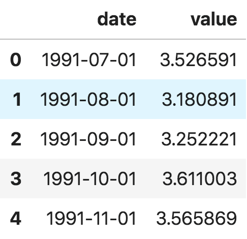

Dataframe Time Series — Dataframe Time Serial

Alternately, you tin import it as a pandas Series with the date as alphabetize. You just demand to specify the index_col argument in the pd.read_csv() to do this.

          ser = pd.read_csv('https://raw.githubusercontent.com/selva86/datasets/primary/a10.csv', parse_dates=['date'], index_col='date') ser.head()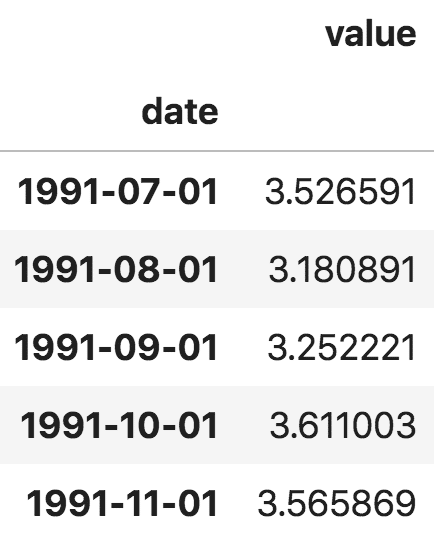

Note, in the serial, the 'value' column is placed college than date to imply that it is a series.

3. What is console information?

Console data is also a fourth dimension based dataset. The difference is that, in improver to time series, it also contains i or more related variables that are measured for the aforementioned time periods. Typically, the columns present in console data incorporate explanatory variables that can be helpful in predicting the Y, provided those columns volition exist available at the time to come forecasting period. An example of panel data is shown below.

          # dataset source: https://github.com/rouseguy df = pd.read_csv('https://raw.githubusercontent.com/selva86/datasets/master/MarketArrivals.csv') df = df.loc[df.market=='Bombay', :] df.head()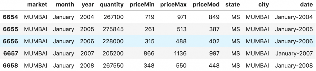

four. Visualizing a time series

Permit'southward use matplotlib to visualise the series.

          # Time series information source: fpp pacakge in R. import matplotlib.pyplot as plt df = pd.read_csv('https://raw.githubusercontent.com/selva86/datasets/primary/a10.csv', parse_dates=['date'], index_col='date')  # Depict Plot def plot_df(df, x, y, title="", xlabel='Date', ylabel='Value', dpi=100):     plt.figure(figsize=(16,five), dpi=dpi)     plt.plot(x, y, color='tab:crimson')     plt.gca().set(title=title, xlabel=xlabel, ylabel=ylabel)     plt.prove()  plot_df(df, 10=df.index, y=df.value, title='Monthly anti-diabetic drug sales in Australia from 1992 to 2008.')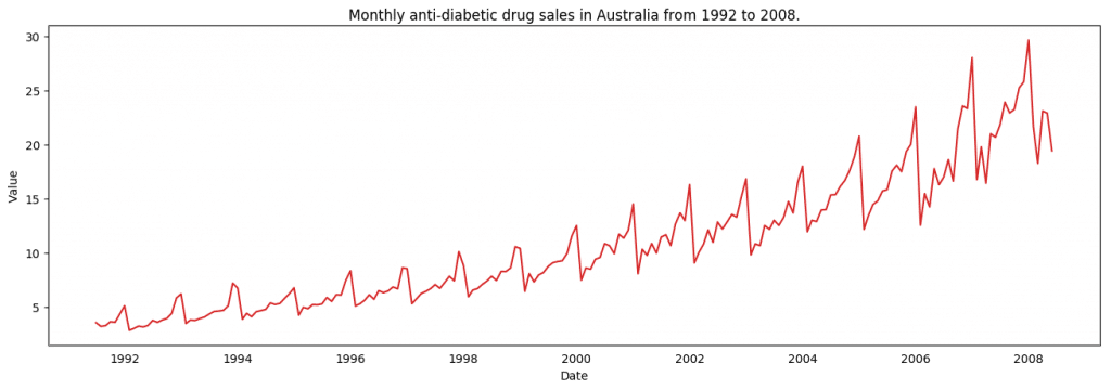

Visualizing Time Series — Visualizing Fourth dimension Series

Since all values are positive, you tin can show this on both sides of the Y centrality to emphasize the growth.

          # Import information df = pd.read_csv('datasets/AirPassengers.csv', parse_dates=['date']) x = df['date'].values y1 = df['value'].values  # Plot fig, ax = plt.subplots(1, 1, figsize=(sixteen,5), dpi= 120) plt.fill_between(x, y1=y1, y2=-y1, alpha=0.five, linewidth=2, colour='seagreen') plt.ylim(-800, 800) plt.title('Air Passengers (Ii Side View)', fontsize=sixteen) plt.hlines(y=0, xmin=np.min(df.engagement), xmax=np.max(df.date), linewidth=.five) plt.show()

Air Passengers Data - 2 Side Series — Air Passengers Information – 2 Side Series

Since its a monthly time serial and follows a certain repetitive pattern every year, you can plot each year as a separate line in the same plot. This lets you compare the twelvemonth wise patterns side-past-side. Seasonal Plot of a Time Serial

          # Import Information df = pd.read_csv('https://raw.githubusercontent.com/selva86/datasets/master/a10.csv', parse_dates=['date'], index_col='date') df.reset_index(inplace=Truthful)  # Gear up data df['year'] = [d.year for d in df.engagement] df['month'] = [d.strftime('%b') for d in df.appointment] years = df['year'].unique()  # Prep Colors np.random.seed(100) mycolors = np.random.choice(list(mpl.colors.XKCD_COLORS.keys()), len(years), replace=Simulated)  # Draw Plot plt.figure(figsize=(sixteen,12), dpi= 80) for i, y in enumerate(years):     if i > 0:                 plt.plot('month', 'value', information=df.loc[df.yr==y, :], color=mycolors[i], label=y)         plt.text(df.loc[df.year==y, :].shape[0]-.nine, df.loc[df.yr==y, 'value'][-1:].values[0], y, fontsize=12, colour=mycolors[i])  # Decoration plt.gca().prepare(xlim=(-0.3, xi), ylim=(2, 30), ylabel='$Drug Sales$', xlabel='$Month$') plt.yticks(fontsize=12, alpha=.7) plt.title("Seasonal Plot of Drug Sales Time Series", fontsize=20) plt.show()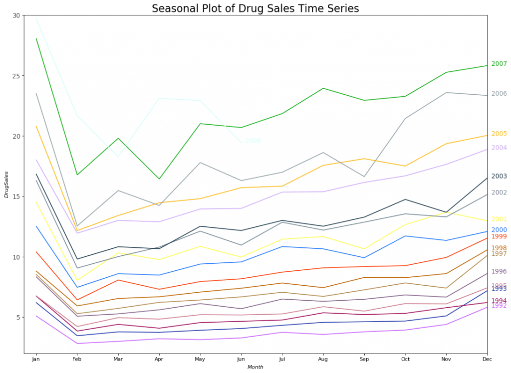

There is a steep fall in drug sales every February, ascent once more in March, falling again in April and so on. Conspicuously, the design repeats within a given year, every yr. However, as years progress, the drug sales increase overall. You tin nicely visualize this trend and how information technology varies each year in a dainty twelvemonth-wise boxplot. Likewise, you can do a month-wise boxplot to visualize the monthly distributions. Boxplot of Month-wise (Seasonal) and Year-wise (tendency) Distribution You can grouping the data at seasonal intervals and see how the values are distributed inside a given twelvemonth or month and how information technology compares over time.

          # Import Information df = pd.read_csv('https://raw.githubusercontent.com/selva86/datasets/main/a10.csv', parse_dates=['date'], index_col='date') df.reset_index(inplace=True)  # Set up data df['twelvemonth'] = [d.yr for d in df.date] df['month'] = [d.strftime('%b') for d in df.date] years = df['year'].unique()  # Draw Plot fig, axes = plt.subplots(1, 2, figsize=(20,7), dpi= lxxx) sns.boxplot(x='year', y='value', data=df, ax=axes[0]) sns.boxplot(ten='month', y='value', data=df.loc[~df.year.isin([1991, 2008]), :])  # Set Title axes[0].set_title('Year-wise Box Plot\n(The Trend)', fontsize=xviii);  axes[1].set_title('Month-wise Box Plot\northward(The Seasonality)', fontsize=18) plt.bear witness()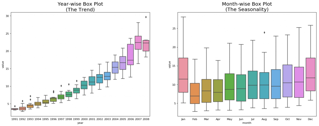

The boxplots make the yr-wise and month-wise distributions evident. As well, in a month-wise boxplot, the months of December and January clearly has higher drug sales, which can be attributed to the vacation discounts season. So far, nosotros have seen the similarities to identify the pattern. At present, how to find out any deviations from the usual pattern?

5. Patterns in a time series

Any time series may be split into the following components: Base Level + Trend + Seasonality + Fault A trend is observed when there is an increasing or decreasing slope observed in the time series. Whereas seasonality is observed when at that place is a distinct repeated pattern observed between regular intervals due to seasonal factors. It could be because of the month of the twelvemonth, the day of the month, weekdays or even time of the 24-hour interval. Yet, It is not mandatory that all time series must accept a trend and/or seasonality. A time serial may not accept a distinct trend merely have a seasonality. The opposite can also be truthful. So, a time series may be imagined every bit a combination of the tendency, seasonality and the error terms.

          fig, axes = plt.subplots(i,3, figsize=(20,four), dpi=100) pd.read_csv('https://raw.githubusercontent.com/selva86/datasets/master/guinearice.csv', parse_dates=['date'], index_col='appointment').plot(title='Trend Just', fable=False, ax=axes[0])  pd.read_csv('https://raw.githubusercontent.com/selva86/datasets/master/sunspotarea.csv', parse_dates=['appointment'], index_col='appointment').plot(title='Seasonality Only', legend=False, ax=axes[i])  pd.read_csv('https://raw.githubusercontent.com/selva86/datasets/master/AirPassengers.csv', parse_dates=['date'], index_col='date').plot(title='Trend and Seasonality', legend=Faux, ax=axes[ii])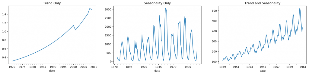

Patterns in Time Series — Patterns in Time Serial

Another aspect to consider is the cyclic behaviour. It happens when the ascension and fall pattern in the series does not happen in stock-still calendar-based intervals. Care should be taken to not confuse 'cyclic' event with 'seasonal' effect. So, How to diffentiate between a 'cyclic' vs 'seasonal' pattern? If the patterns are not of fixed calendar based frequencies, then it is cyclic. Because, dissimilar the seasonality, circadian furnishings are typically influenced past the business and other socio-economic factors.

half-dozen. Additive and multiplicative fourth dimension series

Depending on the nature of the trend and seasonality, a time series tin be modeled as an additive or multiplicative, wherein, each observation in the series can be expressed as either a sum or a product of the components: Additive time series: Value = Base Level + Trend + Seasonality + Error Multiplicative Time Series: Value = Base Level x Trend x Seasonality ten Error

vii. How to decompose a fourth dimension series into its components?

You can do a classical decomposition of a time series past because the series as an additive or multiplicative combination of the base of operations level, trend, seasonal index and the residual. The seasonal_decompose in statsmodels implements this conveniently.

          from statsmodels.tsa.seasonal import seasonal_decompose from dateutil.parser import parse  # Import Information df = pd.read_csv('https://raw.githubusercontent.com/selva86/datasets/primary/a10.csv', parse_dates=['date'], index_col='date')  # Multiplicative Decomposition  result_mul = seasonal_decompose(df['value'], model='multiplicative', extrapolate_trend='freq')  # Condiment Decomposition result_add = seasonal_decompose(df['value'], model='additive', extrapolate_trend='freq')  # Plot plt.rcParams.update({'figure.figsize': (10,ten)}) result_mul.plot().suptitle('Multiplicative Decompose', fontsize=22) result_add.plot().suptitle('Additive Decompose', fontsize=22) plt.show()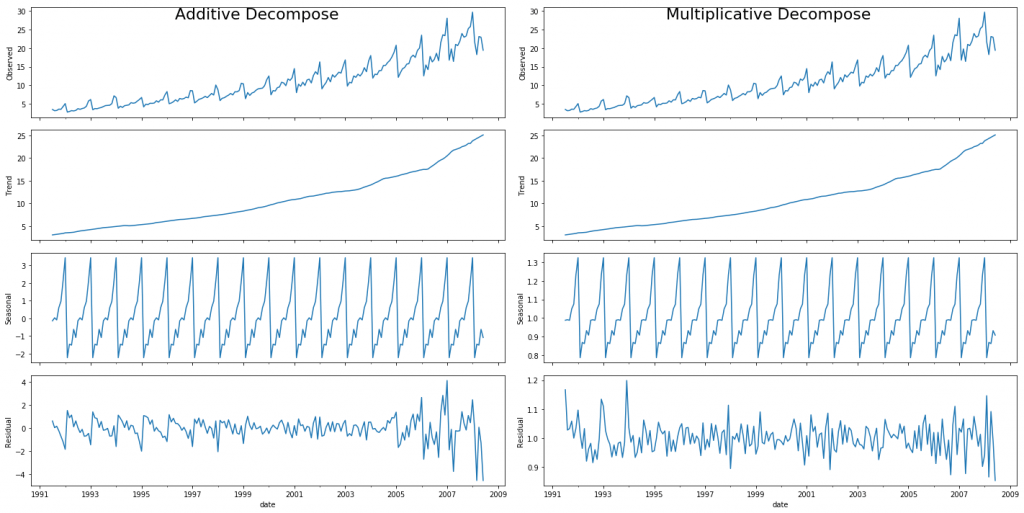

Setting extrapolate_trend='freq' takes intendance of any missing values in the trend and residuals at the beginning of the series. If y'all expect at the residuals of the additive decomposition closely, it has some blueprint left over. The multiplicative decomposition, still, looks quite random which is good. And then ideally, multiplicative decomposition should exist preferred for this particular series. The numerical output of the trend, seasonal and residual components are stored in the result_mul output itself. Allow's extract them and put information technology in a dataframe.

          # Extract the Components ---- # Actual Values = Product of (Seasonal * Trend * Resid) df_reconstructed = pd.concat([result_mul.seasonal, result_mul.trend, result_mul.resid, result_mul.observed], axis=one) df_reconstructed.columns = ['seas', 'trend', 'resid', 'actual_values'] df_reconstructed.caput()

If you check, the product of seas, tendency and resid columns should exactly equal to the actual_values.

8. Stationary and Non-Stationary Fourth dimension Series

Stationarity is a property of a time series. A stationary series is one where the values of the series is not a role of time. That is, the statistical backdrop of the serial similar mean, variance and autocorrelation are constant over fourth dimension. Autocorrelation of the serial is nix but the correlation of the series with its previous values, more than on this coming up. A stationary time series id devoid of seasonal effects every bit well. So how to identify if a series is stationary or not? Let's plot some examples to make it clear:

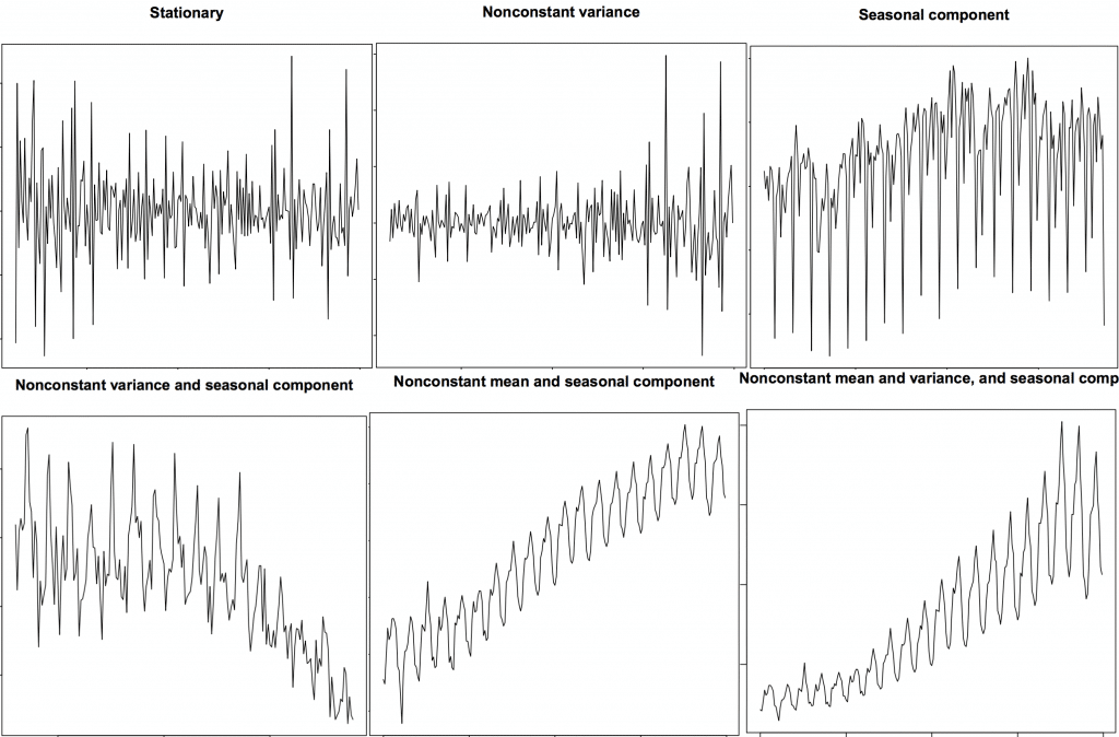
Stationary and Non-Stationary Time Series

The higher up image is sourced from R's `TSTutorial`. So why does a stationary serial thing? why am I even talking about it? I will come up to that in a bit, but sympathize that it is possible to make nearly any time series stationary by applying a suitable transformation. Nearly statistical forecasting methods are designed to work on a stationary time serial. The first step in the forecasting process is typically to do some transformation to convert a non-stationary serial to stationary.

9. How to make a fourth dimension series stationary?

You can make serial stationary by:

Differencing the Series (once or more)
Take the log of the serial
Take the nth root of the series
Combination of the in a higher place

The most mutual and convenient method to stationarize the series is by differencing the series at to the lowest degree once until information technology becomes approximately stationary. So what is differencing? If Y_t is the value at fourth dimension 't', and so the first deviation of Y = Yt – Yt-ane. In simpler terms, differencing the serial is nix but subtracting the next value by the current value. If the first divergence doesn't make a serial stationary, you tin can become for the second differencing. And so on. For case, consider the following serial: [1, five, 2, 12, 20] First differencing gives: [5-ane, 2-v, 12-2, 20-12] = [4, -3, ten, eight] 2nd differencing gives: [-3-4, -ten-iii, viii-10] = [-vii, -13, -ii]

9. Why brand a non-stationary series stationary before forecasting?

Forecasting a stationary series is relatively easy and the forecasts are more reliable. An important reason is, autoregressive forecasting models are substantially linear regression models that utilize the lag(s) of the series itself as predictors. We know that linear regression works best if the predictors (X variables) are not correlated confronting each other. So, stationarizing the serial solves this problem since it removes any persistent autocorrelation, thereby making the predictors(lags of the series) in the forecasting models almost independent. Now that nosotros've established that stationarizing the series important, how do you check if a given serial is stationary or not?

10. How to exam for stationarity?

The stationarity of a series can be established past looking at the plot of the serial like we did earlier. Another method is to separate the series into ii or more face-to-face parts and calculating the summary statistics like the mean, variance and the autocorrelation. If the stats are quite different, then the series is not likely to be stationary. Nevertheless, you need a method to quantitatively determine if a given serial is stationary or not. This can be washed using statistical tests called 'Unit of measurement Root Tests'. In that location are multiple variations of this, where the tests bank check if a time series is non-stationary and possess a unit root. There are multiple implementations of Unit Root tests similar:

Augmented Dickey Fuller exam (ADH Test)
Kwiatkowski-Phillips-Schmidt-Shin – KPSS test (tendency stationary)
Philips Perron test (PP Test)

The most commonly used is the ADF test, where the zero hypothesis is the time series possesses a unit root and is non-stationary. And so, id the P-Value in ADH examination is less than the significance level (0.05), you reject the zilch hypothesis. The KPSS exam, on the other manus, is used to examination for trend stationarity. The nix hypothesis and the P-Value interpretation is merely the reverse of ADH examination. The below code implements these two tests using statsmodels package in python.

          from statsmodels.tsa.stattools import adfuller, kpss df = pd.read_csv('https://raw.githubusercontent.com/selva86/datasets/master/a10.csv', parse_dates=['date'])  # ADF Test consequence = adfuller(df.value.values, autolag='AIC') print(f'ADF Statistic: {result[0]}') print(f'p-value: {result[1]}') for cardinal, value in event[iv].items():     print('Critial Values:')     print(f'   {primal}, {value}')  # KPSS Test upshot = kpss(df.value.values, regression='c') impress('\nKPSS Statistic: %f' % effect[0]) print('p-value: %f' % consequence[1]) for key, value in result[3].items():     print('Critial Values:')     impress(f'   {key}, {value}')

          ADF Statistic: 3.14518568930674 p-value: 1.0 Critial Values:    1%, -iii.465620397124192 Critial Values:    5%, -2.8770397560752436 Critial Values:    10%, -two.5750324547306476  KPSS Statistic: 1.313675 p-value: 0.010000 Critial Values:    10%, 0.347 Critial Values:    5%, 0.463 Critial Values:    2.5%, 0.574 Critial Values:    1%, 0.739

eleven. What is the deviation between white racket and a stationary series?

Like a stationary series, the white noise is also non a function of time, that is its mean and variance does not alter over time. But the difference is, the white racket is completely random with a mean of 0. In white noise there is no pattern whatsoever. If y'all consider the sound signals in an FM radio as a time series, the blank audio y'all hear between the channels is white noise. Mathematically, a sequence of completely random numbers with mean nix is a white noise.

          randvals = np.random.randn(g) pd.Series(randvals).plot(title='Random White Noise', colour='thousand')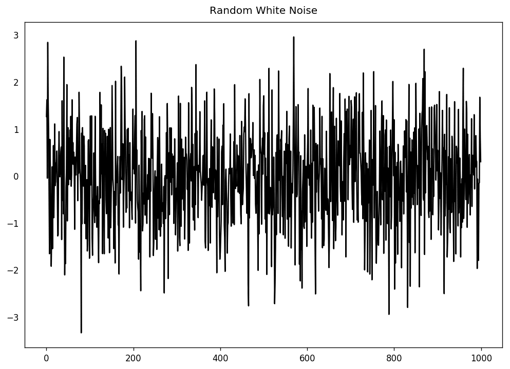

12. How to detrend a time series?

Detrending a time serial is to remove the trend component from a time serial. But how to extract the tendency? In that location are multiple approaches.

Subtract the line of best fit from the time series. The line of best fit may be obtained from a linear regression model with the time steps as the predictor. For more circuitous trends, you may want to use quadratic terms (ten^2) in the model.
Decrease the trend component obtained from time series decomposition we saw earlier.
Subtract the mean
Utilise a filter like Baxter-Male monarch filter(statsmodels.tsa.filters.bkfilter) or the Hodrick-Prescott Filter (statsmodels.tsa.filters.hpfilter) to remove the moving average trend lines or the cyclical components.

Allow's implement the first two methods.

          # Using scipy: Subtract the line of best fit from scipy import signal df = pd.read_csv('https://raw.githubusercontent.com/selva86/datasets/master/a10.csv', parse_dates=['date']) detrended = bespeak.detrend(df.value.values) plt.plot(detrended) plt.championship('Drug Sales detrended by subtracting the least squares fit', fontsize=16)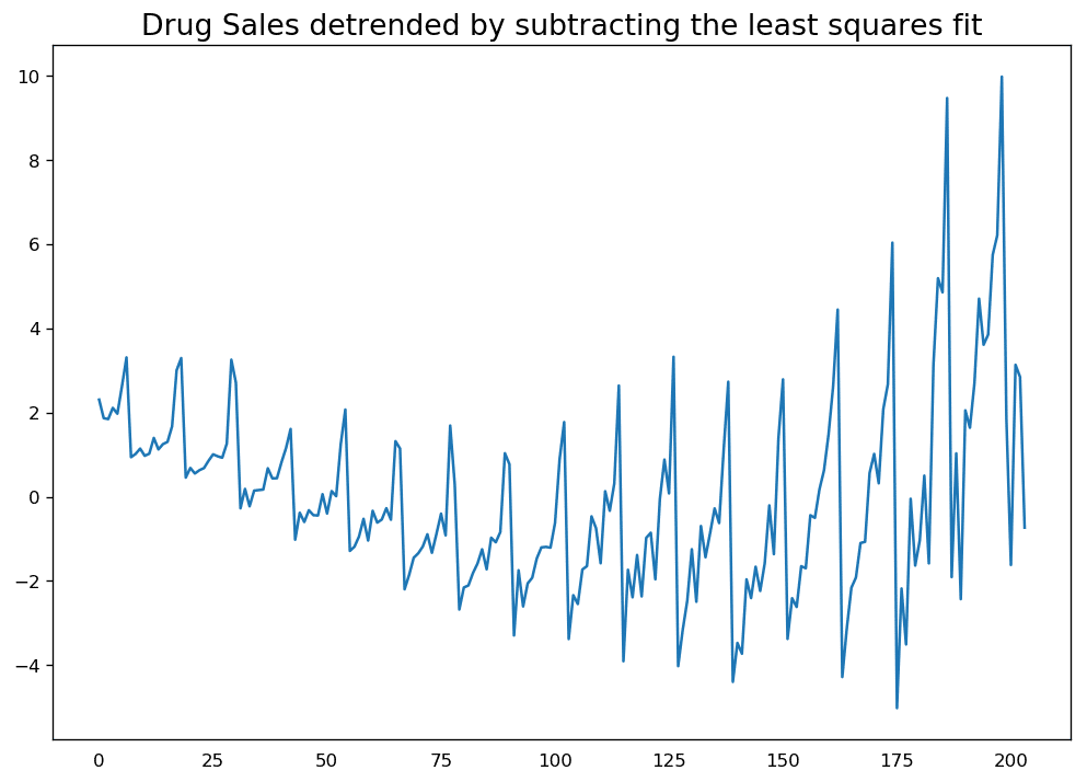

Detrend A TimeSeries By Subtracting LeastSquaresFit

          # Using statmodels: Subtracting the Trend Component. from statsmodels.tsa.seasonal import seasonal_decompose df = pd.read_csv('https://raw.githubusercontent.com/selva86/datasets/master/a10.csv', parse_dates=['date'], index_col='appointment') result_mul = seasonal_decompose(df['value'], model='multiplicative', extrapolate_trend='freq') detrended = df.value.values - result_mul.tendency plt.plot(detrended) plt.title('Drug Sales detrended by subtracting the trend component', fontsize=16)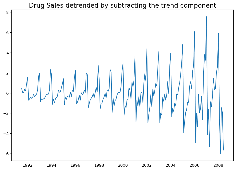

Detrend By Subtracting Trend Component — Detrend By Subtracting Tendency Component

13. How to deseasonalize a time serial?

There are multiple approaches to deseasonalize a time series likewise. Beneath are a few:

          - ane. Take a moving average with length equally the seasonal window. This will shine in series in the procedure.  - 2. Seasonal difference the serial (subtract the value of previous season from the current value)  - 3. Divide the series by the seasonal index obtained from STL decomposition

If dividing past the seasonal alphabetize does non work well, endeavor taking a log of the series and and so do the deseasonalizing. You can later restore to the original scale past taking an exponential.

          # Subtracting the Trend Component. df = pd.read_csv('https://raw.githubusercontent.com/selva86/datasets/master/a10.csv', parse_dates=['date'], index_col='date')  # Time Serial Decomposition result_mul = seasonal_decompose(df['value'], model='multiplicative', extrapolate_trend='freq')  # Deseasonalize deseasonalized = df.value.values / result_mul.seasonal  # Plot plt.plot(deseasonalized) plt.championship('Drug Sales Deseasonalized', fontsize=16) plt.plot()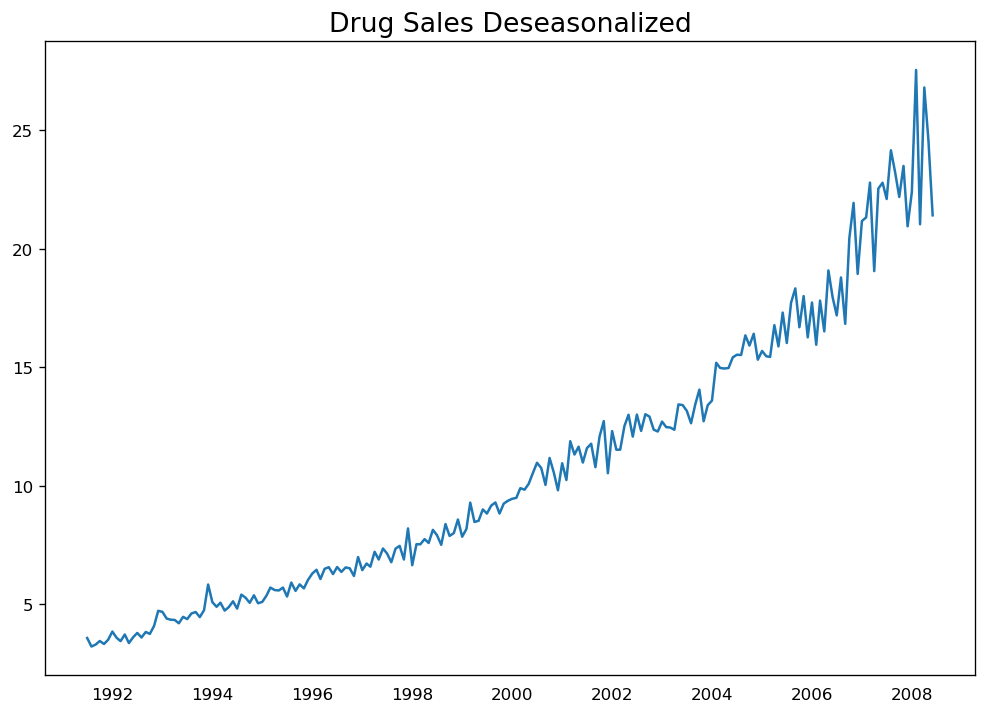

xiv. How to examination for seasonality of a time series?

The common way is to plot the serial and bank check for repeatable patterns in fixed time intervals. So, the types of seasonality is adamant by the clock or the calendar:

Hour of twenty-four hours
Day of month
Weekly
Monthly
Yearly

However, if you lot want a more than definitive inspection of the seasonality, utilise the Autocorrelation Function (ACF) plot. More on the ACF in the upcoming sections. Merely when in that location is a strong seasonal blueprint, the ACF plot commonly reveals definitive repeated spikes at the multiples of the seasonal window. For instance, the drug sales time series is a monthly series with patterns repeating every year. And so, you tin can see spikes at 12th, 24th, 36th.. lines. I must caution you that in real discussion datasets such strong patterns is hardly noticed and can get distorted by any dissonance, then yous demand a conscientious eye to capture these patterns.

          from pandas.plotting import autocorrelation_plot df = pd.read_csv('https://raw.githubusercontent.com/selva86/datasets/master/a10.csv')  # Draw Plot plt.rcParams.update({'figure.figsize':(9,5), 'figure.dpi':120}) autocorrelation_plot(df.value.tolist())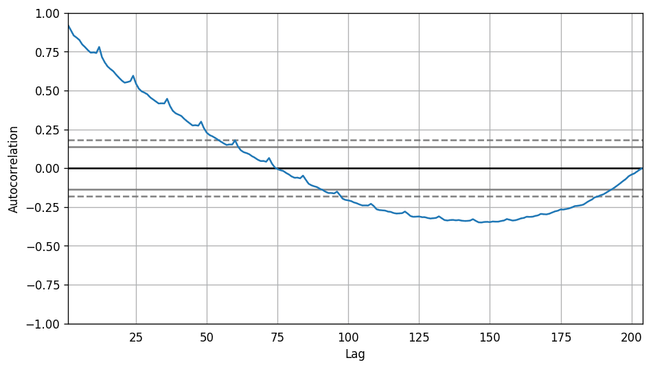

Alternately, if yous want a statistical test, the CHTest can determine if seasonal differencing is required to stationarize the series.

xv. How to treat missing values in a time series?

Sometimes, your time series will have missing dates/times. That ways, the data was non captured or was non bachelor for those periods. It could so happen the measurement was zero on those days, in which case, case you may make full up those periods with zero. Secondly, when it comes to time series, you should typically NOT replace missing values with the mean of the series, particularly if the series is not stationary. What you could practice instead for a quick and muddied workaround is to forrard-fill the previous value. Yet, depending on the nature of the series, you want to endeavour out multiple approaches before final. Some effective alternatives to imputation are:

Backward Make full
Linear Interpolation
Quadratic interpolation
Mean of nearest neighbors
Mean of seasonal couterparts

To measure out the imputation performance, I manually innovate missing values to the fourth dimension series, impute it with to a higher place approaches and and so measure the hateful squared mistake of the imputed against the actual values.

          # # Generate dataset from scipy.interpolate import interp1d from sklearn.metrics import mean_squared_error df_orig = pd.read_csv('https://raw.githubusercontent.com/selva86/datasets/chief/a10.csv', parse_dates=['date'], index_col='engagement').head(100) df = pd.read_csv('datasets/a10_missings.csv', parse_dates=['appointment'], index_col='engagement')  fig, axes = plt.subplots(seven, one, sharex=True, figsize=(x, 12)) plt.rcParams.update({'xtick.bottom' : Imitation})  ## one. Actual ------------------------------- df_orig.plot(title='Bodily', ax=axes[0], label='Actual', color='red', style=".-") df.plot(title='Actual', ax=axes[0], characterization='Bodily', color='dark-green', style=".-") axes[0].fable(["Missing Data", "Bachelor Data"])  ## two. Forward Fill -------------------------- df_ffill = df.ffill() error = np.circular(mean_squared_error(df_orig['value'], df_ffill['value']), ii) df_ffill['value'].plot(championship='Forwards Fill (MSE: ' + str(fault) +")", ax=axes[ane], characterization='Forward Fill', mode=".-")  ## 3. Backward Fill up ------------------------- df_bfill = df.bfill() fault = np.round(mean_squared_error(df_orig['value'], df_bfill['value']), 2) df_bfill['value'].plot(title="Backward Fill (MSE: " + str(mistake) +")", ax=axes[two], label='Dorsum Fill', colour='firebrick', style=".-")  ## iv. Linear Interpolation ------------------ df['rownum'] = np.arange(df.shape[0]) df_nona = df.dropna(subset = ['value']) f = interp1d(df_nona['rownum'], df_nona['value']) df['linear_fill'] = f(df['rownum']) error = np.round(mean_squared_error(df_orig['value'], df['linear_fill']), 2) df['linear_fill'].plot(title="Linear Fill (MSE: " + str(error) +")", ax=axes[3], label='Cubic Fill', colour='brown', style=".-")  ## v. Cubic Interpolation -------------------- f2 = interp1d(df_nona['rownum'], df_nona['value'], kind='cubic') df['cubic_fill'] = f2(df['rownum']) error = np.round(mean_squared_error(df_orig['value'], df['cubic_fill']), 2) df['cubic_fill'].plot(title="Cubic Make full (MSE: " + str(error) +")", ax=axes[4], label='Cubic Fill', color='red', style=".-")  # Interpolation References: # https://docs.scipy.org/doc/scipy/reference/tutorial/interpolate.html # https://docs.scipy.org/doc/scipy/reference/interpolate.html  ## vi. Mean of 'n' Nearest Past Neighbors ------ def knn_mean(ts, n):     out = np.re-create(ts)     for i, val in enumerate(ts):         if np.isnan(val):             n_by_2 = np.ceil(n/2)             lower = np.max([0, int(i-n_by_2)])             upper = np.min([len(ts)+1, int(i+n_by_2)])             ts_near = np.concatenate([ts[lower:i], ts[i:upper]])             out[i] = np.nanmean(ts_near)     render out  df['knn_mean'] = knn_mean(df.value.values, viii) error = np.round(mean_squared_error(df_orig['value'], df['knn_mean']), two) df['knn_mean'].plot(title="KNN Mean (MSE: " + str(fault) +")", ax=axes[5], label='KNN Mean', color='tomato', alpha=0.5, manner=".-")  ## 7. Seasonal Mean ---------------------------- def seasonal_mean(ts, n, lr=0.7):     """     Compute the mean of respective seasonal periods     ts: 1D array-like of the time series     n: Seasonal window length of the time series     """     out = np.copy(ts)     for i, val in enumerate(ts):         if np.isnan(val):             ts_seas = ts[i-1::-n]  # previous seasons only             if np.isnan(np.nanmean(ts_seas)):                 ts_seas = np.concatenate([ts[i-1::-n], ts[i::n]])  # previous and forward             out[i] = np.nanmean(ts_seas) * lr     return out  df['seasonal_mean'] = seasonal_mean(df.value, northward=12, lr=1.25) error = np.round(mean_squared_error(df_orig['value'], df['seasonal_mean']), 2) df['seasonal_mean'].plot(title="Seasonal Mean (MSE: " + str(error) +")", ax=axes[half-dozen], label='Seasonal Mean', color='blue', alpha=0.5, style=".-")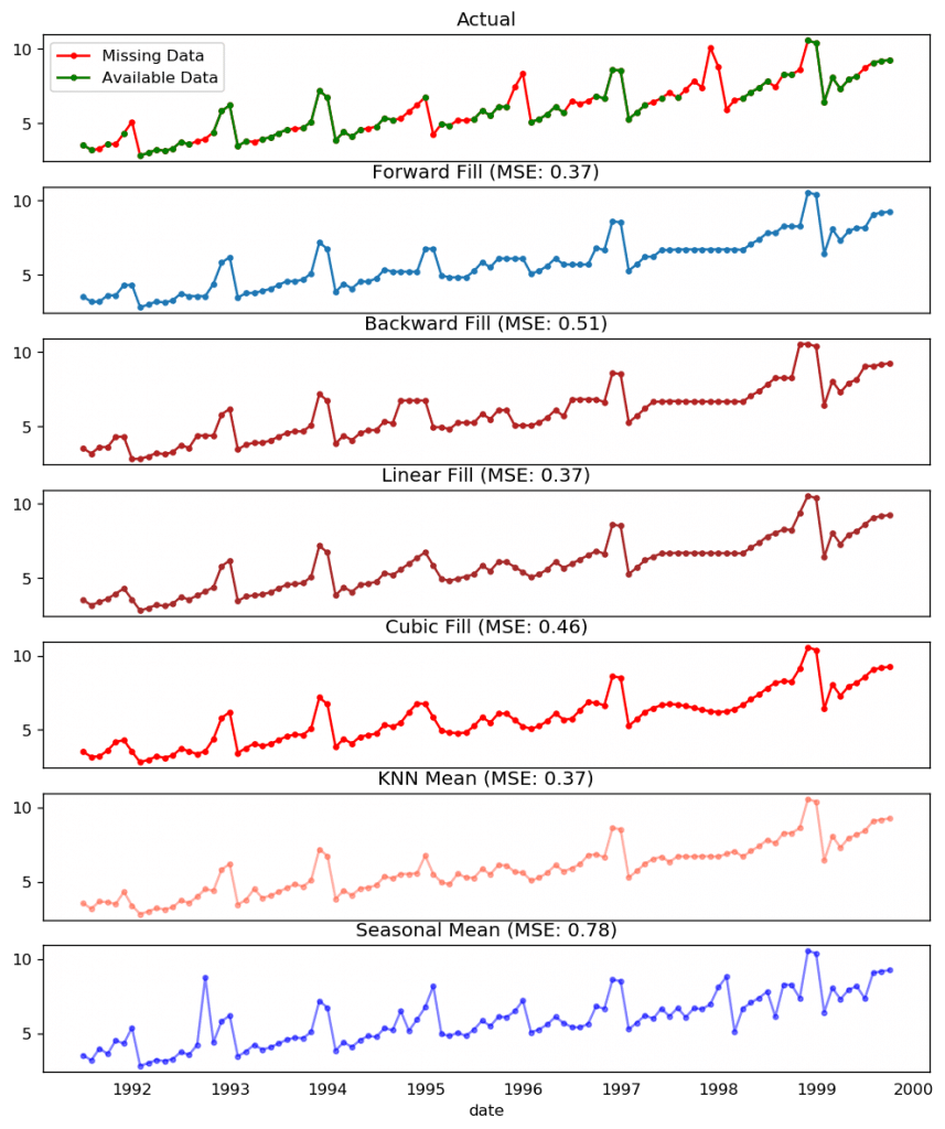

Yous could also consider the following approaches depending on how accurate you want the imputations to exist.

If you have explanatory variables use a prediction model like the random forest or chiliad-Nearest Neighbors to predict it.
If you have enough past observations, forecast the missing values.
If you accept enough hereafter observations, backcast the missing values
Forecast of counterparts from previous cycles.

16. What is autocorrelation and fractional autocorrelation functions?

Autocorrelation is simply the correlation of a serial with its ain lags. If a series is significantly autocorrelated, that ways, the previous values of the series (lags) may be helpful in predicting the current value. Partial Autocorrelation as well conveys similar information just it conveys the pure correlation of a series and its lag, excluding the correlation contributions from the intermediate lags.

          from statsmodels.tsa.stattools import acf, pacf from statsmodels.graphics.tsaplots import plot_acf, plot_pacf  df = pd.read_csv('https://raw.githubusercontent.com/selva86/datasets/master/a10.csv')  # Calculate ACF and PACF upto fifty lags # acf_50 = acf(df.value, nlags=50) # pacf_50 = pacf(df.value, nlags=50)  # Draw Plot fig, axes = plt.subplots(1,2,figsize=(16,3), dpi= 100) plot_acf(df.value.tolist(), lags=50, ax=axes[0]) plot_pacf(df.value.tolist(), lags=50, ax=axes[one])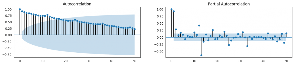

17. How to compute partial autocorrelation part?

So how to compute partial autocorrelation? The partial autocorrelation of lag (k) of a series is the coefficient of that lag in the autoregression equation of Y. The autoregressive equation of Y is nothing but the linear regression of Y with its own lags equally predictors. For Case, if Y_t is the electric current series and Y_t-1 is the lag 1 of Y, then the partial autocorrelation of lag iii (Y_t-iii) is the coefficient $\alpha_3$ of Y_t-3 in the following equation:

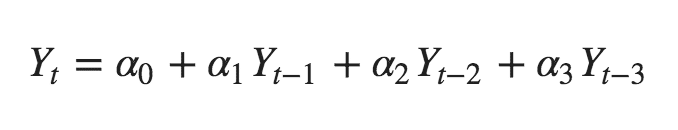
18. Lag Plots

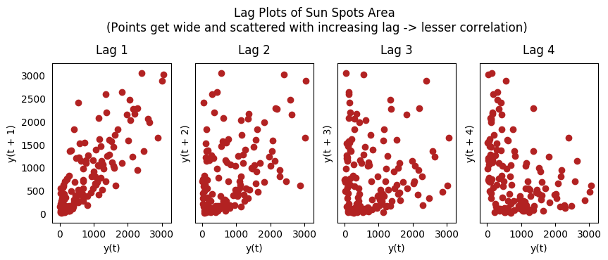
A Lag plot is a scatter plot of a time series against a lag of itself. It is normally used to check for autocorrelation. If there is any design existing in the serial similar the one yous see below, the series is autocorrelated. If there is no such pattern, the series is probable to be random white noise. In beneath instance on Sunspots surface area fourth dimension series, the plots get more and more scattered as the n_lag increases.

          from pandas.plotting import lag_plot plt.rcParams.update({'ytick.left' : False, 'axes.titlepad':ten})  # Import ss = pd.read_csv('https://raw.githubusercontent.com/selva86/datasets/master/sunspotarea.csv') a10 = pd.read_csv('https://raw.githubusercontent.com/selva86/datasets/master/a10.csv')  # Plot fig, axes = plt.subplots(one, 4, figsize=(ten,3), sharex=Truthful, sharey=True, dpi=100) for i, ax in enumerate(axes.flatten()[:iv]):     lag_plot(ss.value, lag=i+one, ax=ax, c='firebrick')     ax.set_title('Lag ' + str(i+1))  fig.suptitle('Lag Plots of Sun Spots Area \n(Points become wide and scattered with increasing lag -> bottom correlation)\n', y=1.xv)      fig, axes = plt.subplots(1, 4, figsize=(x,three), sharex=True, sharey=True, dpi=100) for i, ax in enumerate(axes.flatten()[:four]):     lag_plot(a10.value, lag=i+1, ax=ax, c='firebrick')     ax.set_title('Lag ' + str(i+i))  fig.suptitle('Lag Plots of Drug Sales', y=1.05)     plt.testify()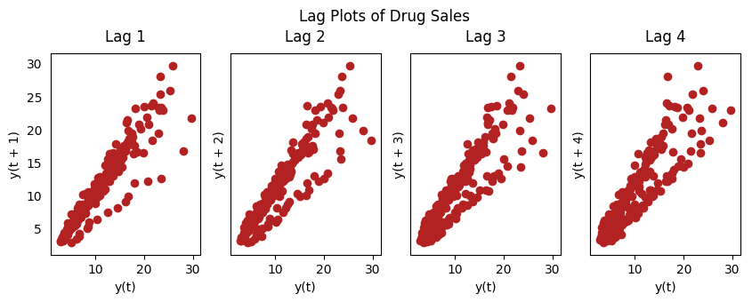

19. How to estimate the forecastability of a time serial?

The more regular and repeatable patterns a time serial has, the easier it is to forecast. The 'Approximate Entropy' tin be used to quantify the regularity and unpredictability of fluctuations in a time series. The higher the judge entropy, the more than hard information technology is to forecast it. Some other amend alternate is the 'Sample Entropy'. Sample Entropy is like to guess entropy just is more than consistent in estimating the complexity fifty-fifty for smaller time serial. For case, a random fourth dimension series with fewer data points tin can accept a lower 'approximate entropy' than a more 'regular' time series, whereas, a longer random time series will take a higher 'approximate entropy'. Sample Entropy handles this problem nicely. Run across the demonstration below.

          # https://en.wikipedia.org/wiki/Approximate_entropy ss = pd.read_csv('https://raw.githubusercontent.com/selva86/datasets/master/sunspotarea.csv') a10 = pd.read_csv('https://raw.githubusercontent.com/selva86/datasets/master/a10.csv') rand_small = np.random.randint(0, 100, size=36) rand_big = np.random.randint(0, 100, size=136)  def ApEn(U, m, r):     """Compute Aproximate entropy"""     def _maxdist(x_i, x_j):         return max([abs(ua - va) for ua, va in naught(x_i, x_j)])      def _phi(one thousand):         x = [[U[j] for j in range(i, i + m - 1 + 1)] for i in range(N - 1000 + 1)]         C = [len([i for x_j in ten if _maxdist(x_i, x_j) <= r]) / (N - chiliad + 1.0) for x_i in x]         return (Due north - m + i.0)**(-i) * sum(np.log(C))      N = len(U)     return abs(_phi(m+1) - _phi(m))  print(ApEn(ss.value, m=2, r=0.2*np.std(ss.value)))     # 0.651 print(ApEn(a10.value, m=2, r=0.2*np.std(a10.value)))   # 0.537 impress(ApEn(rand_small, m=2, r=0.two*np.std(rand_small))) # 0.143 impress(ApEn(rand_big, m=ii, r=0.2*np.std(rand_big)))     # 0.716

          0.6514704970333534 0.5374775224973489 0.0898376940798844 0.7369242960384561

          # https://en.wikipedia.org/wiki/Sample_entropy def SampEn(U, m, r):     """Compute Sample entropy"""     def _maxdist(x_i, x_j):         return max([abs(ua - va) for ua, va in zip(x_i, x_j)])      def _phi(m):         x = [[U[j] for j in range(i, i + m - 1 + one)] for i in range(N - chiliad + ane)]         C = [len([1 for j in range(len(10)) if i != j and _maxdist(10[i], ten[j]) <= r]) for i in range(len(x))]         render sum(C)      Due north = len(U)     return -np.log(_phi(m+i) / _phi(m))  print(SampEn(ss.value, one thousand=2, r=0.two*np.std(ss.value)))      # 0.78 print(SampEn(a10.value, m=2, r=0.2*np.std(a10.value)))    # 0.41 print(SampEn(rand_small, 1000=two, r=0.two*np.std(rand_small)))  # 1.79 print(SampEn(rand_big, one thousand=2, r=0.2*np.std(rand_big)))      # two.42

          0.7853311366380039 0.41887013457621214 inf 2.181224235989778  del sys.path[0]

twenty. Why and How to smoothen a time series?

Smoothening of a time series may exist useful in:

Reducing the event of noise in a signal go a fair approximation of the noise-filtered series.
The smoothed version of serial can be used every bit a feature to explain the original series itself.
Visualize the underlying trend better

Then how to smoothen a series? Permit'due south discuss the following methods:

Take a moving boilerplate
Practise a LOESS smoothing (Localized Regression)
Do a LOWESS smoothing (Locally Weighted Regression)

Moving average is nada but the average of a rolling window of defined width. But you must choose the window-width wisely, considering, large window-size will over-smooth the series. For example, a window-size equal to the seasonal duration (ex: 12 for a month-wise series), will effectively nullify the seasonal effect. LOESS, brusk for 'LOcalized regrESSion' fits multiple regressions in the local neighborhood of each signal. It is implemented in the statsmodels parcel, where you lot can control the degree of smoothing using frac argument which specifies the pct of data points nearby that should be considered to fit a regression model. Download dataset: Elecequip.csv

          from statsmodels.nonparametric.smoothers_lowess import lowess plt.rcParams.update({'xtick.bottom' : False, 'axes.titlepad':v})  # Import df_orig = pd.read_csv('datasets/elecequip.csv', parse_dates=['date'], index_col='date')  # 1. Moving Average df_ma = df_orig.value.rolling(3, middle=True, closed='both').mean()  # two. Loess Smoothing (v% and 15%) df_loess_5 = pd.DataFrame(lowess(df_orig.value, np.arange(len(df_orig.value)), frac=0.05)[:, 1], index=df_orig.index, columns=['value']) df_loess_15 = pd.DataFrame(lowess(df_orig.value, np.arange(len(df_orig.value)), frac=0.15)[:, 1], index=df_orig.index, columns=['value'])  # Plot fig, axes = plt.subplots(4,ane, figsize=(seven, 7), sharex=True, dpi=120) df_orig['value'].plot(ax=axes[0], color='m', championship='Original Serial') df_loess_5['value'].plot(ax=axes[1], title='Loess Smoothed 5%') df_loess_15['value'].plot(ax=axes[2], championship='Loess Smoothed 15%') df_ma.plot(ax=axes[iii], title='Moving Average (3)') fig.suptitle('How to Smoothen a Time Series', y=0.95, fontsize=14) plt.evidence()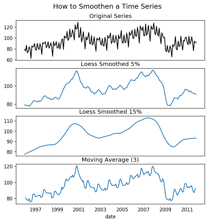

How to use Granger Causality test to know if in one case series is helpful in forecasting another?

Granger causality test is used to determine if i time series will be useful to forecast some other. How does Granger causality test piece of work? It is based on the idea that if X causes Y, then the forecast of Y based on previous values of Y AND the previous values of X should outperform the forecast of Y based on previous values of Y alone. So, understand that Granger causality should non exist used to examination if a lag of Y causes Y. Instead, it is by and large used on exogenous (not Y lag) variables just. It is nicely implemented in the statsmodel package. It accepts a second array with 2 columns as the main argument. The values are in the first column and the predictor (X) is in the second cavalcade. The Cipher hypothesis is: the series in the second column, does not Granger cause the series in the beginning. If the P-Values are less than a significance level (0.05) then yous reject the null hypothesis and conclude that the said lag of X is indeed useful. The second argument maxlag says till how many lags of Y should exist included in the test.

          from statsmodels.tsa.stattools import grangercausalitytests df = pd.read_csv('https://raw.githubusercontent.com/selva86/datasets/main/a10.csv', parse_dates=['appointment']) df['month'] = df.appointment.dt.month grangercausalitytests(df[['value', 'calendar month']], maxlag=2)

          Granger Causality number of lags (no cypher) 1 ssr based F test:         F=54.7797 , p=0.0000  , df_denom=200, df_num=1 ssr based chi2 test:   chi2=55.6014 , p=0.0000  , df=i likelihood ratio examination: chi2=49.1426 , p=0.0000  , df=ane parameter F test:         F=54.7797 , p=0.0000  , df_denom=200, df_num=1  Granger Causality number of lags (no zero) 2 ssr based F test:         F=162.6989, p=0.0000  , df_denom=197, df_num=two ssr based chi2 test:   chi2=333.6567, p=0.0000  , df=two likelihood ratio test: chi2=196.9956, p=0.0000  , df=ii parameter F examination:         F=162.6989, p=0.0000  , df_denom=197, df_num=ii

In the higher up example, the P-Values are Null for all tests. So the 'month' indeed tin be used to forecast the Air Passengers.

22. What Next

That's it for now. We started from the very basics and understood diverse characteristics of a fourth dimension serial. Once the assay is done the side by side step is to begin forecasting. In the next post, I volition walk you through the in-depth procedure of building time serial forecasting models using ARIMA. Run across you soon.

jenkinsplebadve.blogspot.com

Source: https://www.machinelearningplus.com/time-series/time-series-analysis-python/